Jun 07, 2025   Jun 07, 2025

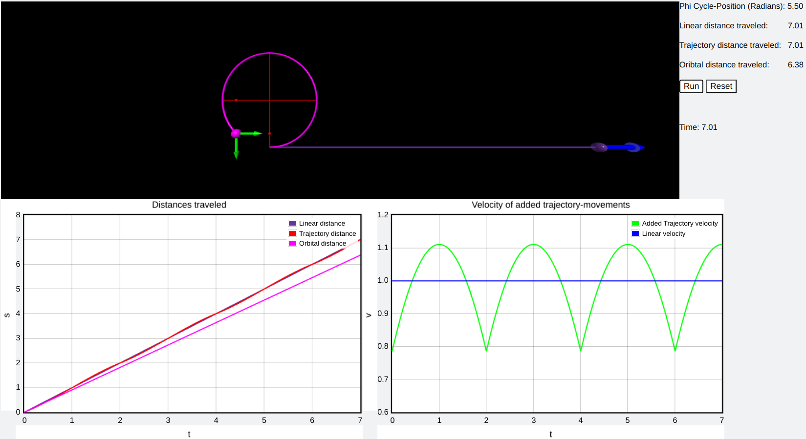
Rotational-kinematical hypothesis and testing of an orbital velocity and distance

A rolling circle on an even path draws a cylcoidal trajectory, which equals the length of 8r, while the traveled distance on the even path equals a length of 2 * pi * r. The fact, that the cycloidal trajectory and the rolled distance on the even path do not equal, begs a question seeing that a fixed point has been followed in both cases (one measured by a xy-background and the other measured by an even line) and thus should be equal, if the rolled distance of a circle (--> 2 * pi * r [green]) measured by the intercept point moving on a straight line (x-axis) would perfectly incorporate a traveled path of a fixed point located on the rolling circle (--> 8r [red]) but measured by a stationary background (xy-coordinate system).

This difference is perfectly explained for any kind of cycloids by the rolling itself. How ? ... by imagining a circle as a polygone consisting of infinite vertices. The sum of these infinite small side lengths equals 2 * pi * r, while rolling creates an additional trajectory caused by rotating on the polygones vertices before the next following polygonal side length touches the roll-path.

Hypothesis

The next and final question , which consequentially rises after studying the rolling process and which shall be the roational-kinematical hypothesis to be tested, is following:

Does a stationary circle (rolling in-place) or an object moving along a circular path also create a trajectory of 8r?

If the answer is Yes, than the drawn (= traveled) circumference of any circular path would equal 8r, while a circumference of 2 * pi * r would only be valid for an already given (= statical) circle with no object on it undergoing circular kinematics

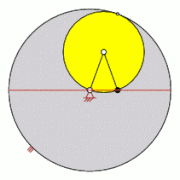
Preparation of the hypothesis (by analyzing the hypocycloid)

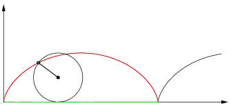
What counts for rolling on an even path (red cycloid on top) is also valid for the rolling-process on a curve (e.g hypocycloid below), by which the traveled distance of 2*8r (=8R) is generated as well (observing the point on the red line) as in following animation:

$$ \begin{aligned} \small \text{Start position } (\theta = 0): \enspace \text{Red point on the most right position} \newline \small f(\theta): \enspace \text{Traveled red trajectory} \newline \small \theta: \enspace \text{Traveled angle of the length between the two center of both circles} \end{aligned} $$

Setting-up the hypocycloidal equation to solve

\[ \begin{gather} f(\theta) = \int_{0}^{2\pi} \sqrt{ \Big({dx \over d\theta}\Big)^2 + \Big({dy \over d\theta}\Big)^2 } \enspace d\theta \newline \sqrt{\Big({dx \over d\theta}\Big)^2 + \Big({dy \over d\theta}\Big)^2} = \sqrt{(R-r)^2 \cdot \Big[2 + 2 \Big(\sin\theta \cdot \sin \Big({R \over r}\theta-\theta \Big)\Big) - 2 \Big(\cos\theta \cdot \cos \Big({R \over r}\theta-\theta \Big)\Big)\Big]} \end{gather} \]

Now we have set-up the full equation we will stop before its analytical solving and directly jump to a method of numerically solving the equation for one rotation of the hypocycloid (one cycle of drawing the red trajectory).

Numerical solving of the hypocycloidal equation (Monte-Carlo-Simulation)

To be continued ...

Results of object-movement on a circular path via VPython

Source Code